Do you need affinity, or do you need kinetics? That one question decides your SPR setup. Manual injection — what we call static SPR — gives you affinity (KD) at steady state, fast and simply. A pump — kinetic SPR — adds continuous flow, so you can watch the complex come apart and measure how fast it forms and breaks (kon, koff) as well as KD.
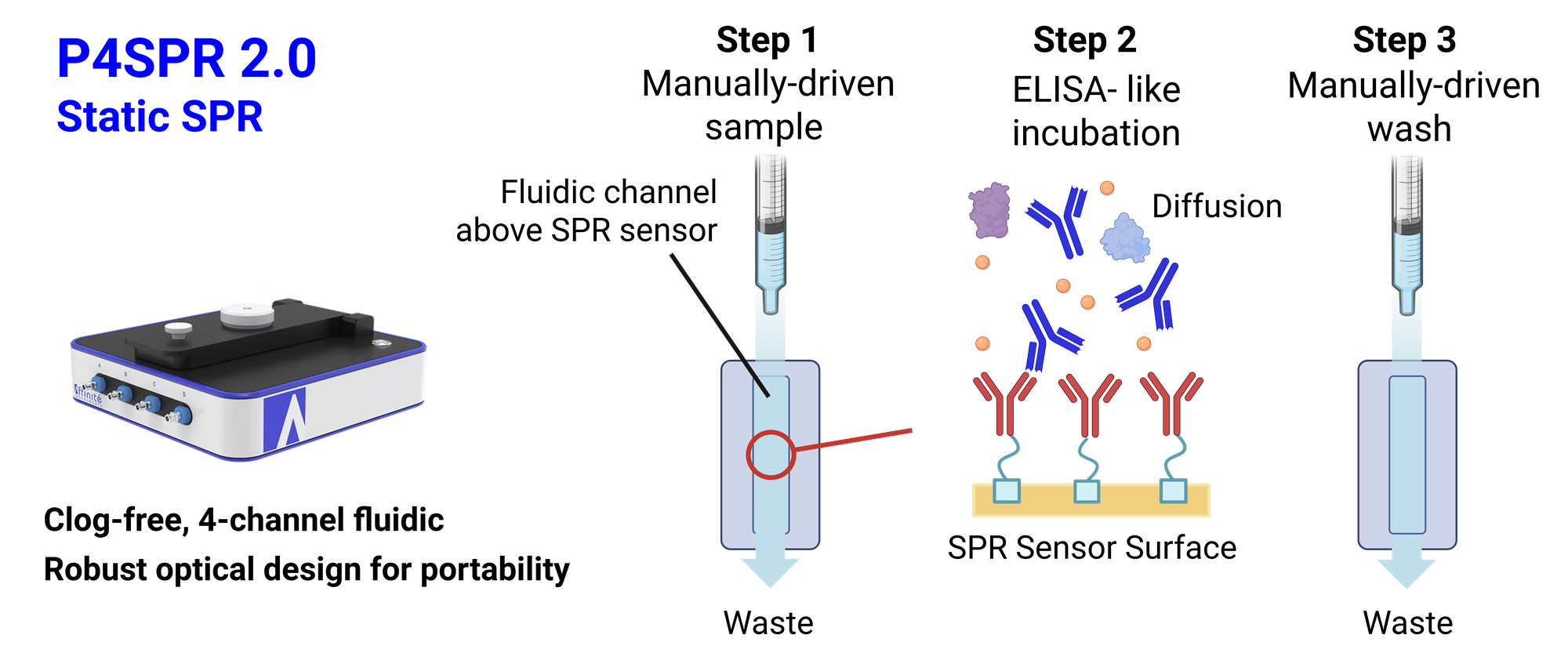
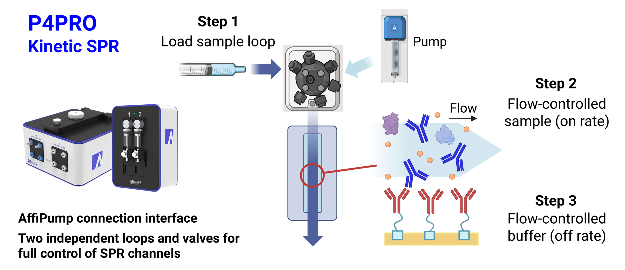
The rest of this guide explains why: how each mode works, what the sensorgrams look like, and how to choose.
Basic Principles of Kinetics and Affinity
In an SPR experiment, ligands (L) are immobilized onto the sensing surface and introduced to an analyte (A). If A has affinity for L at a 1:1 ratio, one can assume a Langmuir binding model:1–3
L + A ⇌ LA (kon, koff)
Here, kon (M−1 s−1) is the association rate constant and koff (s−1) is the dissociation rate constant (also written ka and kd). The dissociation equilibrium constant KD — the point at which half of the surface-immobilized ligands are bound to analytes — can be expressed in terms of the free concentrations of analyte [A], ligand [L], and analyte-ligand complex [AL], and also directly from the rate constants:
KD = [L][A] / [AL] = koff / kon
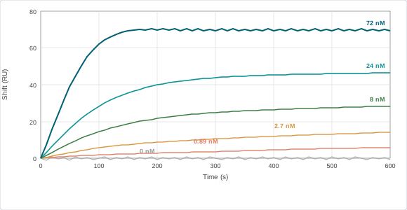
A sensorgram has three main regions used in both steady-state and kinetic experiments. The manual injection mode (steady-state) uses the association region (A) and steady-state plateau (B) to obtain affinity data only. The pump mode (kinetics) uses the association and dissociation phases (A and C) to obtain both kinetic and affinity data.
Manual Injection: Static SPR for Affinity (KD)
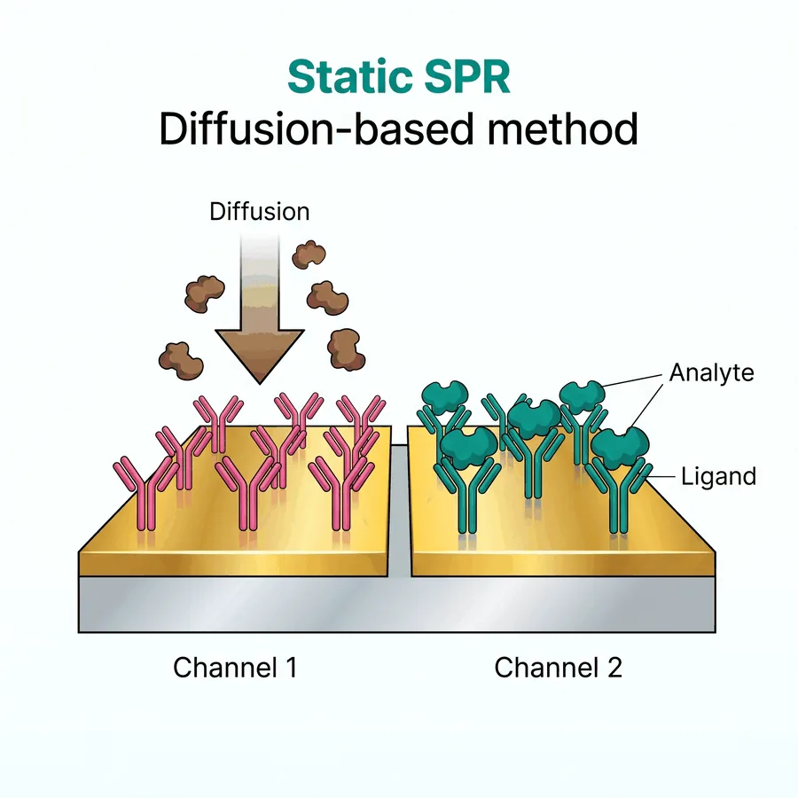
In manual injection mode, samples are injected into the SPR instrument via syringe. Steady-state measurements involve observing equilibrium binding — where the net rate of binding is zero — as a function of analyte concentration, to determine KD.
A typical experiment involves injecting a series of increasing analyte concentrations (at least 5 concentrations) and allowing the sample to remain in contact with the sensor surface until the binding curve levels out (steady state). Note that there is no dissociation phase, since steady-state conditions must be met and there is no flow. The SPR response at steady-state is then plotted against analyte concentration to generate a binding isotherm, and KD is determined by fitting that curve to the steady-state equation.
Pump-Assisted: Kinetic SPR for kon, koff and KD
A pump is required for kinetic measurements because a continuous flow must be provided to observe the dissociation phase following sample injection. The pump delivers sample and running buffer in sequence over the sensor surface. On the P4PRO, the AffiPump does this job.
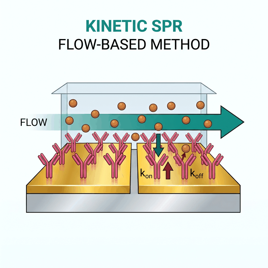
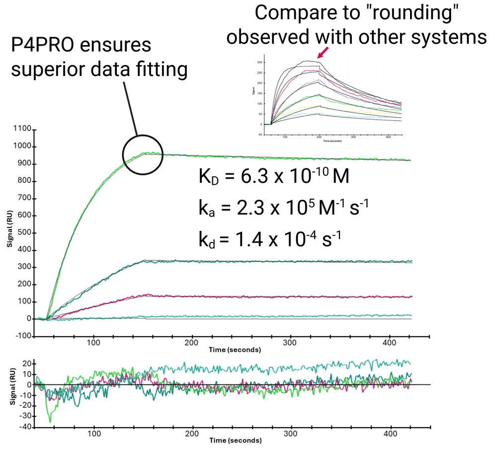
Once the sensorgrams are collected, the association phase is fitted with a suitable binding model — usually a 1:1 Langmuir model (single exponential) — to obtain kon. The dissociation phase is then fitted with a single exponential decay model to find koff. KD is then calculated as KD = koff / kon. The steady-state plateau is not observed in kinetic analysis because running buffer is introduced before the analyte-ligand interaction reaches equilibrium, forcing dissociation.4
Multi-Cycle vs. Single-Cycle Kinetics
Kinetic analysis can be performed in two ways:
Multi-cycle kinetics — one analyte concentration is injected to provide one complete sensorgram, followed by a regeneration step. A new concentration is then injected for the next sensorgram, and so on until all concentrations are run. At least 5–8 concentrations are recommended.
Single-cycle kinetics — multiple analyte concentrations (usually low to high, up to 5 concentrations) are injected within the same cycle with no regeneration steps in between.
In both cases, it is recommended to use a range of concentrations centered around the expected KD (from 0.1 to 10 × KD) to eliminate artifacts due to concentration dependency when fitting to a binding model. Other considerations for kinetic measurements include the requirement for more sample volume and the potential for mass transfer effects at high analyte concentrations.
Which one should you choose? Multi-cycle gives you a separate curve for every concentration, so you can subtract a blank per curve, drop a failed injection and troubleshoot complex binding. Single-cycle is the better choice when regeneration would damage your ligand or surface — or simply when you want a shorter run.
When Static SPR Is the Better Choice
Kinetics is not automatically "better". If the complex dissociates quickly — as a rule of thumb, koff faster than about 10−3 s−1 — binding reaches steady state fast and the plateau gives a reliable KD. Once dissociation gets faster than about 10−1 s−1, the rate constants become hard to resolve at all, and steady-state analysis is the way to go. This is common with small molecules and fragments.2
Steady-state is also a useful cross-check: if the KD from the plateau agrees with koff/kon from your kinetic fit, you can trust the result more.2
Comparison Summary
| Manual injection (static) | Pump-assisted (kinetic) | |
|---|---|---|
| Measurement type | Steady-state | Kinetic |
| Data obtained | KD (affinity) | kon, koff, KD (kinetics + affinity) |
| Flow | No continuous flow | Continuous flow required |
| Dissociation phase | Not observed | Observed and fitted |
| Sample volume | Low | Higher |
| Equipment needed | Syringe only | SPR instrument + pump |
| Mass transfer effects | None | Possible at high concentrations |
| Portability | Maximum — no accessories required | Reduced — pump required |
| Affinité instrument | P4SPR 2.0 | P4PRO + AffiPump |
Besides the type of data needed, factors such as cost, sample volume, time, and portability all influence which setup is most appropriate for a given experiment. On time, static wins: our TN-05 comparison puts static assays at up to half the time of kinetic SPR.
Two Instruments, Both Modes
Affinité Instruments builds one instrument for each need — and both run the same sensors and the same software, so your methods carry over. Researchers have published binding studies on Affinité's portable SPR — for example protein–heparin interactions5 and the effect of serum albumin on binding kinetics6 — and portable SPR as a whole is reviewed in reference 7.
_edited.jpg)
Keep reading
- Static vs Kinetic cheat sheet (one-page reference)
- SPR Sensorgram Explained — how to read the curves above, including a signal that never returns to baseline
References
- P. A. van der Merwe, "Surface Plasmon Resonance," in S. E. Harding and B. Z. Chowdhry (eds.), Protein–Ligand Interactions: Hydrodynamics and Calorimetry — A Practical Approach, Oxford University Press, 2001. PDF (archived copy)
- P. Schuck, "Use of surface plasmon resonance to probe the equilibrium and dynamic aspects of interactions between biological macromolecules," Annual Review of Biophysics and Biomolecular Structure 26 (1997) 541–566. doi:10.1146/annurev.biophys.26.1.541
- J. Homola, "Surface plasmon resonance sensors for detection of chemical and biological species," Chemical Reviews 108 (2008) 462–493. doi:10.1021/cr068107d
- S. Hearty, P. Leonard, H. Ma and R. O'Kennedy, "Measuring antibody–antigen binding kinetics using surface plasmon resonance," in Antibody Engineering: Methods and Protocols (3rd ed.), Methods in Molecular Biology, Springer, 2018, 421–455. doi:10.1007/978-1-4939-8648-4_22
- D. Su, Y. Li, E. Yates, M. Skidmore, M. Lima and D. Fernig, "Analysis of protein–heparin interactions using a portable SPR instrument," PeerJ Analytical Chemistry 4 (2022) e15. doi:10.7717/peerj-achem.15
- B. Charron, A. Delorme, C. Dubois, M. Hojjat Jodaylami and J.-F. Masson, "Influence of bovine and human serum albumin on the binding kinetics of biomolecular interactions," Analyst 148 (2023) 5525–5533. doi:10.1039/D3AN01117H
- J.-F. Masson, "Portable and field-deployed surface plasmon resonance and plasmonic sensors," Analyst 145 (2020) 3776–3800. doi:10.1039/D0AN00316F