The sensorgram is the core output of every SPR experiment — a real-time plot of binding signal versus time. Understanding what each phase represents is the foundation of interpreting SPR data correctly.
What Is a Sensorgram?
When molecules bind to a surface, they change the local refractive index near that surface. SPR detects this change optically and reports it as a signal, typically expressed in Response Units (RU) or millidegrees. Plotting this signal continuously over the course of an experiment produces the sensorgram.
What is a Response Unit (RU)?
An RU is a tiny change in refractive index at the sensor surface. That change scales with the mass bound to the surface,2 so the signal tells you how much material has attached — a widely used rule of thumb is that 1 RU corresponds to roughly 1 pg of protein per mm². The practical consequence: big molecules give big signals. An antibody can produce hundreds of RU, while a small molecule occupying the same number of sites may give only a handful.
Because the measurement is continuous and label-free, the sensorgram captures the full kinetics of the interaction — not just an endpoint. This is what makes SPR fundamentally different from techniques like ELISA, which only report whether binding occurred, not how fast it formed or fell apart.
The Five Phases of a Sensorgram
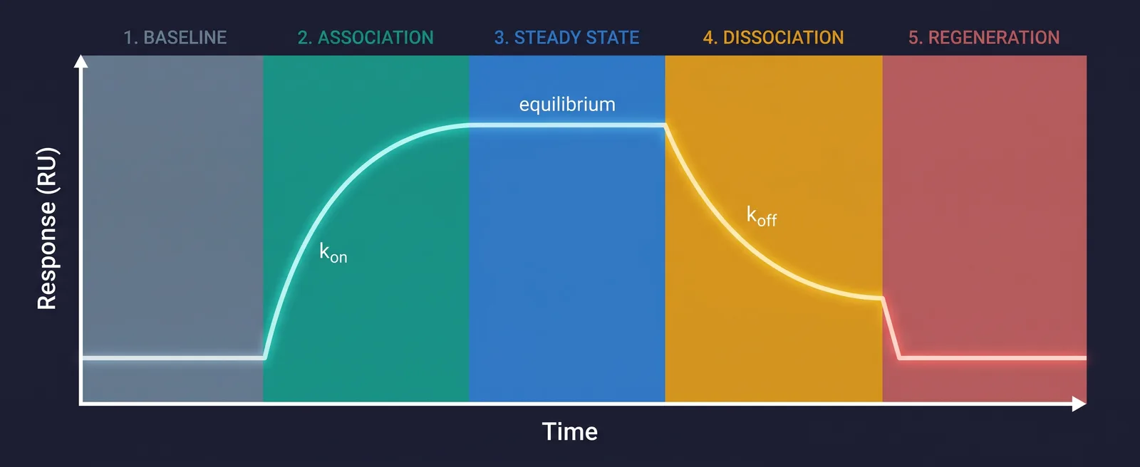
1. Baseline. Before any sample is introduced, a running buffer flows over the sensor surface. This establishes a stable reference signal. A flat, stable baseline is essential — drift or noise here will propagate through the entire experiment.
2. Association phase. The analyte sample is injected and flows over the ligand-coated sensor surface. As binding occurs, the refractive index increases and the signal rises. The rate at which the signal rises reflects both the association rate constant (kon, also written ka) and the analyte concentration. A steep rise on its own does not mean high affinity: affinity (KD = koff / kon) also depends on how quickly the complex falls apart.
3. Equilibrium / steady state. If the association and dissociation rates balance out during the injection window, the signal plateaus. This plateau level is concentration-dependent and is used in steady-state affinity analysis to determine the equilibrium dissociation constant (KD).
4. Dissociation phase. Running buffer replaces the sample, and the bound analyte begins to dissociate from the surface. The signal decreases at a rate determined by the dissociation rate constant (koff, also written kd). A slow dissociation (flat curve) indicates tight binding; a rapid drop indicates a weaker or transient interaction. If the curve is almost perfectly flat, run a longer dissociation phase so koff can be fitted reliably.
5. Regeneration. In most experiments, a regeneration solution is briefly applied to remove any remaining bound analyte and return the surface to baseline — ready for the next injection. Choosing the right regeneration condition (pH, salt, detergent) without damaging the ligand surface is a critical part of assay development.
What Can You Extract from a Sensorgram?
A well-designed SPR experiment produces sensorgrams at multiple analyte concentrations. Fitting these curves to a binding model yields:3
- kon (association rate constant, M−1s−1) — how fast the complex forms
- koff (dissociation rate constant, s−1) — how fast the complex breaks apart
- KD (equilibrium dissociation constant, M) — overall binding affinity, calculated as koff / kon
- Rmax — the maximum binding capacity of the surface, useful for surface quality assessment
- Concentration — via calibration curve, the analyte concentration in an unknown sample
Kinetic vs. Steady-State Analysis
There are two main approaches to extracting affinity data from sensorgrams. Kinetic analysis fits the full shape of the association and dissociation curves simultaneously to extract kon and koff individually — this gives the most complete picture of binding behavior. Steady-state analysis uses only the equilibrium plateau levels at each concentration and fits them to a binding isotherm to get KD directly. Steady-state is simpler and works well for fast-dissociating interactions where true equilibrium is reached during the injection window.1 It is also what static SPR on the P4SPR 2.0 measures — Manual injection vs pump-assisted SPR explains when KD alone is enough.
Reading the Shape: What Can Go Wrong
Not every sensorgram looks like a textbook curve. These are four of the most common shapes — open any card for the causes and the fix.
 Baseline drifting
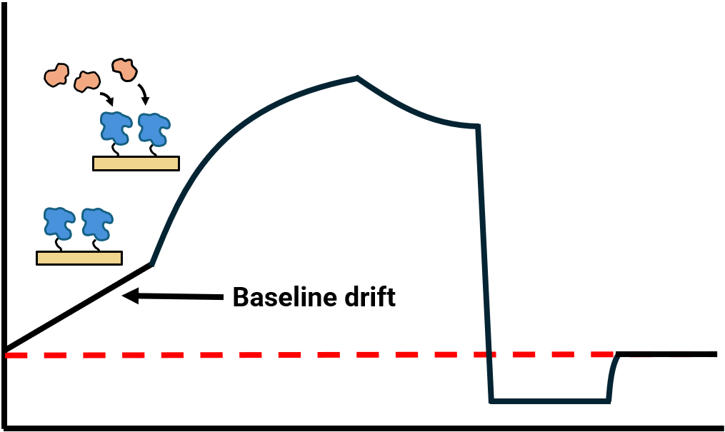
Baseline Drift
A gradual upward or downward drift during the run, often from temperature changes or an unstable sensor surface.
Causes & fix →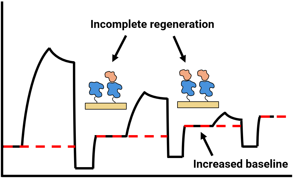 Baseline rising
Incomplete Surface Regeneration
Analyte isn’t fully cleared between cycles, so the baseline steps up and binding capacity drops.
Causes & fix →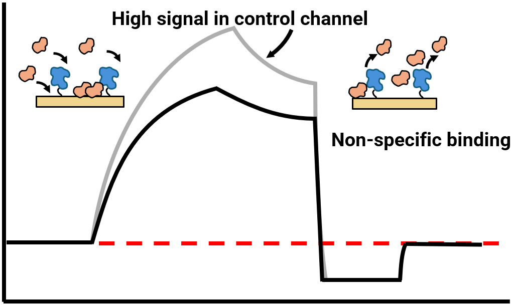 High signal
Non-Specific Binding
The analyte sticks to the surface itself: a high signal in the reference channel that isn’t real binding.
Causes & fix →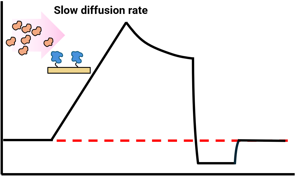 Poor model fit
Mass Transport Limitation
Analyte reaches the surface slower than it binds, so the rise looks linear and depends on flow rate.
Causes & fix →See all 14 patterns in the Sensorgram Pattern Guide →
Bulk Shift or Real Binding?
One of the most common surprises: a square-shaped jump the instant the sample goes in, and an equally sudden drop the instant buffer comes back. That is usually not binding. It is a bulk refractive-index effect — the sample simply has a slightly different refractive index from the running buffer. A little extra salt, DMSO or glycerol is enough.
How to tell them apart: real binding curves in and out gradually and changes with concentration in a way that levels off; a bulk shift is instant, flat-topped and vanishes the moment you switch back to buffer. The fix is to match your sample buffer to the running buffer as closely as you can — and to subtract a reference channel. Dr. Live has taken this question more than once on the Ask Dr. Live forum.
Why the Reference Channel Matters
Everything that is not specific binding — bulk shifts, drift, analyte sticking to the surface itself — shows up in every channel. So you record it in a reference channel (a surface without the ligand, or with an irrelevant one) and subtract it from the active channel. Subtracting a buffer-only (blank) injection as well removes what is left; this is called double referencing, and it is standard practice for clean kinetics.3
It is also why the P4SPR 2.0 has four simultaneous channels: you can run your sample and its controls in the same injection.
Conclusion
The sensorgram packs a remarkable amount of information into a single time-resolved plot. Once you understand the five phases and what each parameter means, you can move quickly from raw data to meaningful conclusions about binding affinity, kinetics, and surface quality. The Affinité SPR platform is designed to generate clean, reproducible sensorgrams with minimal setup — so you can focus on interpreting the biology, not troubleshooting the instrument. Portable benchtop SPR of this kind is now well established in the research literature.4
References
- P. Schuck, "Use of surface plasmon resonance to probe the equilibrium and dynamic aspects of interactions between biological macromolecules," Annual Review of Biophysics and Biomolecular Structure 26 (1997) 541–566. doi:10.1146/annurev.biophys.26.1.541
- J. Homola, "Surface plasmon resonance sensors for detection of chemical and biological species," Chemical Reviews 108 (2008) 462–493. doi:10.1021/cr068107d
- S. Hearty, P. Leonard, H. Ma and R. O'Kennedy, "Measuring antibody–antigen binding kinetics using surface plasmon resonance," in Antibody Engineering: Methods and Protocols (3rd ed.), Methods in Molecular Biology, Springer, 2018, 421–455. doi:10.1007/978-1-4939-8648-4_22
- J.-F. Masson, "Portable and field-deployed surface plasmon resonance and plasmonic sensors," Analyst 145 (2020) 3776–3800. doi:10.1039/D0AN00316F