What does KD mean in SPR?

KD is the equilibrium dissociation constant, expressed in molar units (M, nM, µM). It is the analyte concentration at which half of the immobilized ligands are bound at equilibrium, and in a 1:1 binding model KD = koff / kon. The lower the KD, the tighter the interaction.

What is the difference between kinetic and steady-state SPR for measuring KD?

Kinetic (flow) SPR records both association and dissociation in real time; fitting the curves globally yields kon, koff, Rmax and KD = koff / kon. Steady-state analysis uses only the plateau of each sensorgram, plotted against concentration, and returns Rmax and KD but not the individual rate constants; it works well when the interaction reaches equilibrium within the injection window. The P4SPR 2.0 runs in static mode and determines KD from the steady-state concentration-response curve; the P4PRO with the AffiPump runs both static and kinetic experiments and delivers kon, koff, KD and Rmax.

What analyte concentrations should I use for an SPR affinity experiment?

Aim for roughly 0.1× to 10× the expected KD. A serial dilution, for example three-fold steps across five concentrations, gives well-separated curves that can be fitted reliably. If every concentration is too high the surface saturates immediately; if every concentration is too low the signal is negligible. If the KD is unknown, run a wide scouting series first.

Why does my SPR baseline creep up or drift down between cycles?

Check that the baseline returns to the same level after each regeneration. A baseline that creeps up means analyte is not fully removed and material is accumulating on the surface (regeneration too mild). One that drifts down means ligand is being stripped or damaged (regeneration too harsh). A common regeneration solution is low-pH glycine, e.g. 10 mM glycine-HCl, pH 2.5; scout milder or harsher conditions if needed.

How do you reduce non-specific binding in SPR?

Signal on the reference surface, or binding that never dissociates, points to a sticky analyte or surface. Use reference subtraction, add a surfactant such as Tween 20 (typically 0.005–0.05%) to the running buffer, and block unused surface groups after immobilization.

SPR Binding Affinity: Measuring KD for Protein

Q: How do you measure binding affinity (KD) with SPR?

Run a concentration series around the expected KD with reference and blank subtraction, then either fit the association and dissociation curves (kinetic KD = koff / kon) or fit the plateau responses against concentration (steady-state KD). Check data quality before fitting.

← Back to Blog

How tightly do your two proteins bind — and how fast do they find each other and let go? SPR answers both in real time, without labels. This guide covers how to set up the experiment, the two ways to get K_D, how to design the assay so the numbers hold up, and what bad data looks like. New to sensorgrams? Start with SPR Sensorgram Explained.

SPR Assay Setup

Setting up an SPR experiment for examining protein-protein interactions involves attaching a capture protein molecule onto the SPR sensor chip surface. Then, the protein of interest (the analyte) is injected into a microfluidic channel, which is in contact with the sensor chip. As the analyte flows into the channel, it starts binding to the capture protein, causing the refractive index to change. Depending on the experimental setup, the resultant SPR sensorgram is used to extract information about the specificity, concentration, affinity, and/or association and dissociation rate of the protein-protein interaction.¹

A note on terms used below: the ligand is the recognition element immobilized on the sensor surface (here, the capture protein), and the analyte is the binding partner in solution that you inject over it.

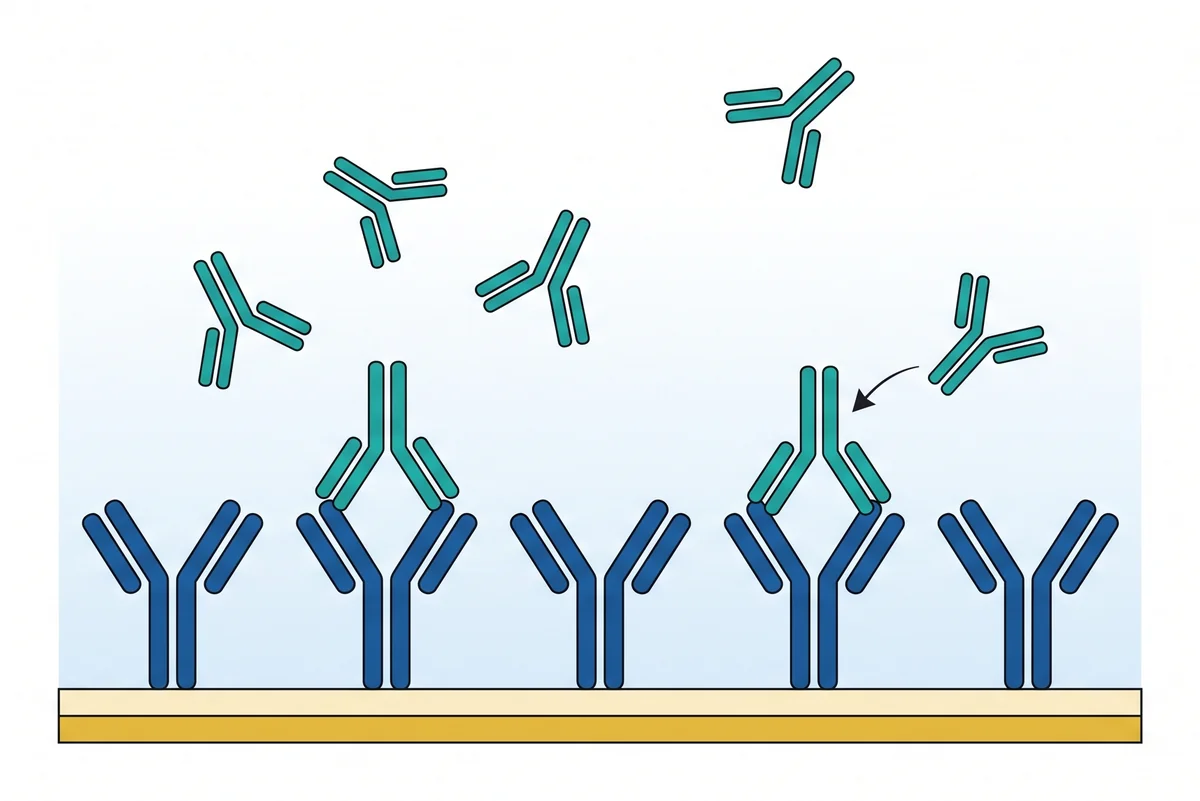
Blue anti-human IgG antibodies anchored on a gold sensor surface capture teal human IgG molecules from the solution above — Ligand on the surface, analyte in solution: here an anti-human IgG antibody (blue, the ligand) captures human IgG (teal, the analyte). The same pair is used in the figures below.

What Binding Affinity (K_D) Means in SPR

Binding affinity describes how tightly two proteins hold on to each other. In SPR it is reported as the equilibrium dissociation constant, K_D, expressed in molar units (M, nM, µM). Using the basic 1:1 (Langmuir) binding model, where an immobilized ligand (L) binds an analyte (A):

A + L ⇌ AL K_D = k_off / k_on

k_on (also written k_a, association rate constant, M⁻¹s⁻¹) — how fast the complex forms.
k_off (also written k_d, dissociation rate constant, s⁻¹) — how fast the complex falls apart.
K_D (M) — the analyte concentration at which half of the immobilized ligands are bound at equilibrium. The lower the K_D, the tighter the interaction.

Because K_D is a ratio, two interactions can share the same affinity yet behave very differently: one may bind and release quickly, the other may bind slowly and stay bound for a long time. That difference is only visible when k_on and k_off are measured separately.

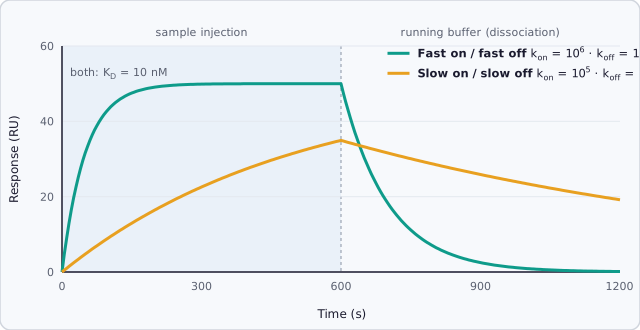
Two simulated sensorgrams with the same KD of 10 nM: the fast pair reaches its plateau quickly and falls back quickly; the slow pair rises slowly and is still bound long after the injection — Same affinity, different behaviour (simulated, 1:1 model, both injected at 10 nM). Both pairs have K_D = 10 nM, but one forms and falls apart in seconds while the other is still largely bound ten minutes later. k_on in M⁻¹s⁻¹, k_off in s⁻¹.

Two Ways to Measure K_D with SPR

SPR gives you affinity in one of two ways, depending on how the experiment is run. Both start from sensorgrams recorded at several analyte concentrations.²

1. Kinetic analysis (association and dissociation fitting)

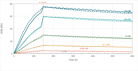
In kinetic (flow) SPR, analyte is delivered over the surface under constant flow and then replaced by running buffer, so both the association and dissociation phases are recorded in real time. The rise of the signal during injection reflects k_on (together with analyte concentration); the decay after injection reflects k_off. Fitting the full set of curves globally to a binding model yields k_on, k_off, R_max and a quantitative K_D = k_off / k_on. This gives the most complete picture of the interaction, including how long a complex lasts once formed.

2. Steady-state (equilibrium) analysis

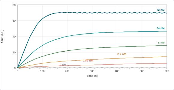
In steady-state analysis you only use the plateau of each sensorgram — the point where association and dissociation balance and the signal stops changing. Plot the plateau response against analyte concentration and fit the resulting binding curve: the fit returns R_max and K_D, which corresponds to the concentration giving half of R_max. Individual rate constants are not obtained. Steady-state analysis is simpler and works well when the interaction reaches true equilibrium within the injection window. In static SPR, where only the association phase is observed, the result is often described as an apparent K_D from a concentration titration.

Kinetic SPR: human IgG at 0 to 72 nM binding immobilized anti-human IgG, association then dissociation after the switch to buffer — One protein–protein pair, measured both ways: human IgG (0–72 nM) binding an immobilized anti-human IgG antibody. Left, kinetic mode — the red dashed line marks the switch to buffer, so both binding and release are fitted. Right, static mode — each concentration climbs to its own plateau, and the plateau heights give K_D.

Static SPR: the same concentrations each rise to their own plateau, with no dissociation phase — One protein–protein pair, measured both ways: human IgG (0–72 nM) binding an immobilized anti-human IgG antibody. Left, kinetic mode — the red dashed line marks the switch to buffer, so both binding and release are fitted. Right, static mode — each concentration climbs to its own plateau, and the plateau heights give K_D.

Which approach should you use?

Static and kinetic SPR are complementary rather than competing. A common workflow is to screen quickly in static mode — yes/no binding, specificity, an affinity estimate — and then characterize the most promising interactions kinetically. In our protein–protein screening application note, four candidate partners were screened in parallel against one immobilized protein, one per channel, in a single run: two bound, two did not. On Affinité's systems, the P4SPR 2.0 runs in static mode (no pump), with four channels for sample and controls in one injection, and determines K_D from the steady-state concentration-response curve. The P4PRO with the AffiPump adds flow-based injection, so it runs both static and kinetic experiments and delivers k_on, k_off, K_D and R_max.

In Affinité's side-by-side comparison of a human IgG / anti-human IgG interaction, static SPR on the P4SPR 2.0 gave K_D ≈ 5 nM and kinetic SPR on the P4PRO gave K_D ≈ 1 nM (k_on = 3.42 × 10⁵ M⁻¹s⁻¹, k_off = 3.10 × 10⁻⁴ s⁻¹). The gap came mainly from the lower-concentration curves not fully reaching steady state in the static run. The full data are in Static vs. Kinetic SPR: P4SPR 2.0 and P4PRO Compared, and the Static vs Kinetic SPR cheat sheet summarizes when to use each mode.

Designing an SPR Binding Affinity Assay

Good affinity numbers come from good assay design. Before you fit anything, make sure the experiment includes the following:³

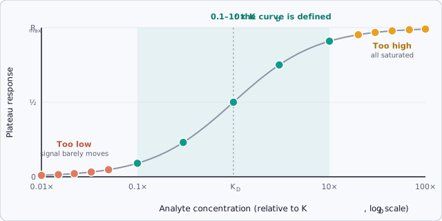
A concentration series spanning the expected K_D. Aim for roughly 0.1× to 10× the expected K_D. If every concentration is too high the surface saturates immediately; if every concentration is too low the signal is negligible. A serial dilution (for example, three-fold steps across five concentrations) gives well-separated curves that can be fitted reliably. If the K_D is unknown, run a wide scouting series first.
A reference channel or surface. Run the same injections over a surface without the specific ligand (or with an irrelevant protein) and subtract it from the active channel. This removes bulk refractive-index shifts and non-specific binding. With multiple channels on one sensor, sample and reference can be measured in the same injection.
A buffer blank. Include a zero-concentration injection of running buffer and subtract it as well. Together, reference and blank subtraction leave only the specific binding signal.
Regeneration between cycles. A short pulse of regeneration solution — often low-pH glycine, e.g. 10 mM glycine-HCl, pH 2.5 (scout milder or harsher conditions if needed) — removes bound analyte and returns the surface to baseline. Check that the baseline returns to the same level each cycle; a baseline that creeps up means analyte is not fully removed (regeneration too mild); one that drifts down means ligand is being stripped or damaged (regeneration too harsh).
Low ligand density for kinetics. Immobilize only as much ligand as you need for a clear signal. High ligand density favors mass transport limitation and rebinding, which distort the association and dissociation curves.
Long enough contact time. For steady-state analysis, inject long enough for every concentration — especially the lowest — to reach a plateau. For kinetic analysis, also record a long enough dissociation phase to see the signal decay clearly.
Replicates. Repeat at least some concentrations. Replicate curves should superimpose.

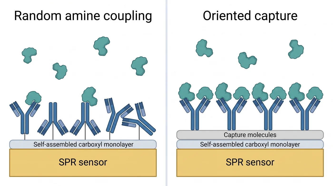
Binding curve on a log concentration axis: concentrations far below KD barely register, far above KD all saturate, and 0.1 to 10 times KD spread across the curve — Why 0.1–10× K_D: concentrations well below K_D barely move the signal, and well above it everything is already saturated. Only a series that spans K_D defines the curve — and therefore K_D itself. (Illustrative, 1:1 binding.)

For protein-protein interactions, it also matters which partner goes on the surface. Immobilizing the smaller or more robust partner and injecting the other is a common starting point, but the best orientation depends on your proteins; testing both configurations, or using a capture approach that orients the ligand, can help. See TN-01: Sensor Surface Functionalization for coupling options.

Random amine coupling leaves antibodies pointing in all directions with few analytes bound; oriented capture holds every antibody upright so more analyte binds — Orientation matters. Random amine coupling attaches the ligand at any lysine, so some binding sites face the surface; a capture layer holds every ligand upright and leaves its binding sites free.

What Good SPR Affinity Data Looks Like — and Common Pitfalls

A dataset you can trust has a flat baseline, association curves with clear curvature (ideally single-exponential), plateaus that climb with concentration and approach saturation at the highest concentrations, a clean dissociation decay, negligible injection spikes, and superimposable replicates. Watch for these problems:

Mass transport limitation. If the association phase looks linear rather than curved, the rate at which analyte reaches the surface — not the binding itself — is controlling the signal. Kinetic constants fitted from such data will be wrong. Lower the ligand density and, in flow mode, increase the flow rate.
Not reaching equilibrium. If the signal is still rising when the injection ends, steady-state analysis will underestimate R_max and overestimate K_D. Extend the contact time, or use kinetic fitting instead.
Non-specific binding. Signal on the reference surface, or binding that never dissociates, points to sticky analyte or surface. Add a surfactant such as Tween 20 (typically 0.005–0.05%) to the running buffer, and block unused surface groups after immobilization.
Curve shapes that do not fit a 1:1 model. Biphasic dissociation can indicate a heterogeneous surface or multiple binding sites; a hook at high concentrations can indicate aggregation. Do not force poor-quality data into a more complex model — improve the surface chemistry, ligand density, regeneration or concentration range first.

For a phase-by-phase guide and a quality checklist, see TN-03: The SPR Sensorgram Explained and the Sensorgram Pattern Guide.

In Short

To measure binding affinity, run a concentration series around the expected K_D with reference and blank subtraction, then either fit the association and dissociation curves (kinetic K_D = k_off / k_on) or fit the plateau responses against concentration (steady-state K_D). Check data quality before fitting, and the numbers you report will hold up. Weighing SPR against other methods? See SPR: advantages and disadvantages.

References

J. Homola, "Surface plasmon resonance sensors for detection of chemical and biological species," Chemical Reviews 108 (2008) 462–493. doi:10.1021/cr068107d
P. Schuck, "Use of surface plasmon resonance to probe the equilibrium and dynamic aspects of interactions between biological macromolecules," Annual Review of Biophysics and Biomolecular Structure 26 (1997) 541–566. doi:10.1146/annurev.biophys.26.1.541
S. Hearty, P. Leonard, H. Ma and R. O'Kennedy, "Measuring antibody–antigen binding kinetics using surface plasmon resonance," in Antibody Engineering: Methods and Protocols (3rd ed.), Methods in Molecular Biology, Springer, 2018, 421–455. doi:10.1007/978-1-4939-8648-4_22

Measuring Binding Affinity with SPR: Protein-Protein Interactions

SPR Assay Setup

What Binding Affinity (K_D) Means in SPR

Two Ways to Measure K_D with SPR

1. Kinetic analysis (association and dissociation fitting)

2. Steady-state (equilibrium) analysis

Which approach should you use?

Designing an SPR Binding Affinity Assay

What Good SPR Affinity Data Looks Like — and Common Pitfalls

In Short

References

See the instrument behind the research.

Measuring Binding Affinity with SPR: Protein-Protein Interactions

SPR Assay Setup

What Binding Affinity (KD) Means in SPR

Two Ways to Measure KD with SPR

1. Kinetic analysis (association and dissociation fitting)

2. Steady-state (equilibrium) analysis

Which approach should you use?

Designing an SPR Binding Affinity Assay

What Good SPR Affinity Data Looks Like — and Common Pitfalls

In Short

References

See the instrument behind the research.

What Binding Affinity (K_D) Means in SPR

Two Ways to Measure K_D with SPR