Affilabs.core
Software
SPR instrument control, data acquisition, and data analysis in one desktop application — from reference-subtracted sensorgrams to steady-state and kinetic fits. Built for the P4SPR and P4PRO, with Sparq smart operation support built right in.
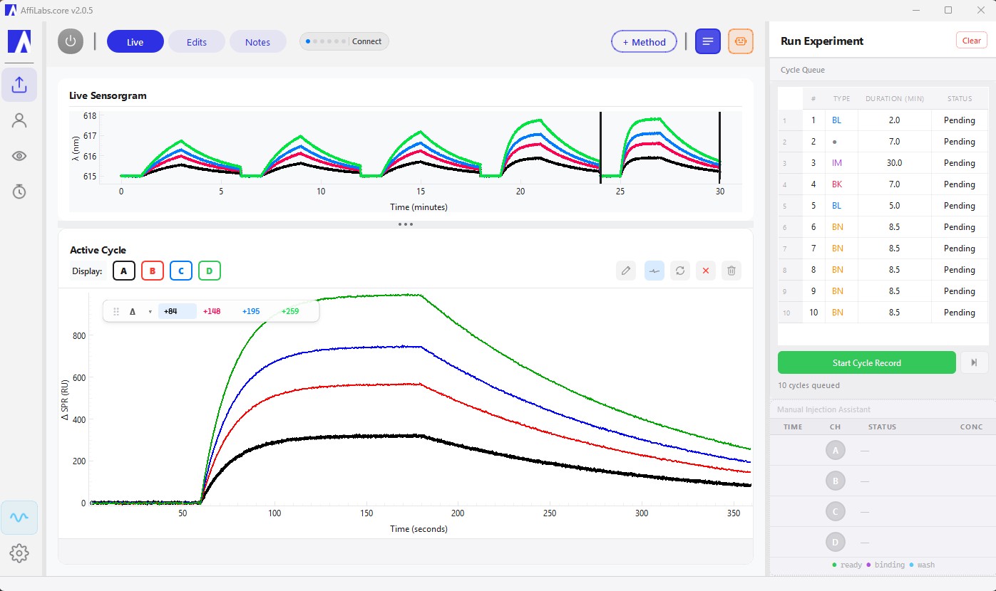
Affilabs.core is the desktop software included with every P4SPR and P4PRO instrument. It controls the instrument, records a live four-channel sensorgram, applies reference-channel subtraction, fits steady-state affinity (KD) and, on P4PRO data, binding kinetics, and exports results to Excel or CSV for Origin and Prism. Sparq, the built-in assistant, flags signal-quality issues during the run.
Live 4-channel wavelength plot with automatic injection flags and cycle markers.
One-click servo alignment, LED calibration, and S-pol reference capture.
Multi-step sequences with templates. Add steps mid-run.
Alignment, ΔSPR cursors, KD fitting, and cycle comparison.
Excel, CSV for Origin and Prism, sensorgram images, clipboard.
Leak and bubble detection with real-time signal quality scoring.
Tag, annotate, rate, and search your experiment history.
Timestamped qualification reports for regulatory and lab audits.
Machine learning optimizes LED settings and convergence automatically.
Live 4-channel wavelength plot with automatic injection flags and cycle markers.
One-click servo alignment, LED calibration, and S-pol reference capture.
Multi-step sequences with templates. Add steps mid-run.
Alignment, ΔSPR cursors, KD fitting, and cycle comparison.
Excel, CSV for Origin and Prism, sensorgram images, clipboard.
Leak and bubble detection with real-time signal quality scoring.
Tag, annotate, rate, and search your experiment history.
Timestamped qualification reports for regulatory and lab audits.
Machine learning optimizes LED settings and convergence automatically.
SPR data analysis
SPR data analysis follows a consistent order: inspect the raw sensorgrams, subtract the reference channel, choose steady-state or kinetic fitting, fit the simplest model (1:1 Langmuir) first, then judge the fit by its residuals and the plausibility of the constants. Common analysis errors come from skipping a step or forcing a complex model onto flawed data.
An SPR sensorgram plots response (RU) against time through five phases: baseline, association, steady state, dissociation and regeneration. The rising association curve reflects binding, its plateau approaches equilibrium, and the decay after the analyte is replaced by buffer reflects dissociation. Before fitting anything, check that the baseline is stable and the curve shapes look plausible.
Walk through each phase in SPR sensorgram explained, and match odd curve shapes to their causes with the sensorgram troubleshooting cheat sheet.
In Affilabs.core: a live 4-channel sensorgram with automatic injection flags and cycle markers, plus real-time signal quality scoring with leak and bubble detection. Sparq, the built-in assistant, also flags common data patterns such as mass transport, bulk refractive-index shifts, drift and incomplete regeneration.
Reference subtraction removes signal that is not specific binding. A reference channel carries the same surface without the ligand, so subtracting it cancels bulk refractive-index shifts from the sample buffer, temperature drift and much of the non-specific binding. Many labs also subtract a buffer-only (blank) injection, known as double referencing, to remove remaining systematic artifacts.
In Affilabs.core: set the reference channel in the Edits tab. On the P4SPR 2.0, four channels run together — three active and one reference. Double referencing (also subtracting a blank buffer injection) is supported.
Fit steady-state affinity when you only need KD: plot the equilibrium response against analyte concentration and fit a binding isotherm for KD and Rmax. Fit kinetics when you need on- and off-rates: fit the association and dissociation curves globally for ka and kd, then KD = kd / ka. Kinetic data need controlled, continuous flow.
Steady-state fitting is only as good as the plateau: each concentration must be at, or very close to, equilibrium when you read the response.
In Affilabs.core: steady-state and kinetic fitting with the basic models: a 1:1 Langmuir isotherm for steady-state KD, and a 1:1 kinetic fit for ka, kd and KD on flow data. The P4SPR 2.0 is a static (steady-state) instrument; the P4PRO with AffiPump adds controlled flow for kinetics. See the Starter Test Kit protocol for a KD fit step by step.
The 1:1 Langmuir model assumes one analyte molecule binds one independent, identical site, which is the simplest possible binding mechanism. It has the fewest fitted parameters, so its constants are the most robust. Start with it, and treat systematic deviations from it as a clue about your assay before reaching for a more complex model.
In Affilabs.core: select the Langmuir 1:1 model in the Binding subtab and click Calculate KD; the fit reports KD, Rmax and R².
Only when independent evidence supports the mechanism. Heterogeneous-ligand, two-state (conformational change) and bivalent-analyte models add parameters, so they almost always fit better than 1:1, even when the mechanism is wrong. Biphasic curves often come from a mixed or overloaded surface, aggregation or mass transport. Fix the surface, ligand density and concentration range first.
Supporting evidence for a complex model includes a known second binding site, a documented conformational change, or the same deviation persisting across ligand densities and surface chemistries. More on this in measuring KD for protein–protein interactions.
Look at the residuals, the difference between data and fit. They should scatter randomly around zero at the noise level; systematic waves mean the model does not describe the data. Also check that fitted values are physically plausible: Rmax consistent with ligand density, and a concentration series spanning 0.1× to 10× KD. A high R² alone is not proof.
In Affilabs.core: residual plots are shown with the fit, R² is reported with the Langmuir 1:1 KD fit, and data export to Excel or CSV for Origin and Prism. For advanced models (heterogeneous ligand, two-state, mass transport), export the data to a specialized fitting tool.
Mass transport limitation occurs when analyte reaches the sensor surface more slowly than it binds, so delivery rather than the interaction controls the signal. Signs include a nearly linear association phase and rate constants that change with flow rate. Reduce ligand density, raise the flow rate, and test two or three flow rates before trusting kinetic constants.
Fitting models with a mass-transport term exist, but they correct for the effect rather than remove it; a well-designed experiment is the better fix.
Multi-cycle kinetics injects one analyte concentration per cycle, with regeneration between cycles, giving one complete sensorgram per concentration. Single-cycle kinetics injects increasing concentrations one after another in a single cycle, with a long dissociation phase at the end and no regeneration in between. Single-cycle suits ligands that are hard to regenerate; both are fitted globally.
For a side-by-side of manual injection and pump-assisted runs, see Manual injection vs pump-assisted SPR.
In Affilabs.core: the Method Queue builds multi-step run sequences from templates, and steps can be added mid-run. Templates cover both single-cycle and multi-cycle kinetics.
Further reading: SPR sensorgram explained · SPR binding affinity for protein–protein interactions · Sensorgram troubleshooting cheat sheet
Sparq
Sparq stands for Surface Plasmon Analysis Result Quality — and Sparq is the smart operation support assistant built directly into Affilabs.core. When something isn't working — or you're not sure what to do next — Sparq walks you through it, step by step, without leaving the application.
No ticket system. No waiting. Just answers.
Full IQ/OQ qualification included with every installation.
Affilabs.core is a Windows desktop application. No internet connection required to run experiments.
Affilabs.core is included with every P4SPR and P4PRO instrument. Get in touch to learn more.
Contact us →Previously using ezControl? That software is no longer supported. Reach out to discuss upgrading to an Affilabs.core-compatible instrument.