Resources · SPR Guide
A plain guide to surface plasmon resonance: the principle behind it, what it measures, how to read a sensorgram, what you need to run an experiment, and how long it takes.
Surface plasmon resonance (SPR) is a label-free optical technique that measures molecules binding to each other in real time. One partner is attached to a thin gold sensor surface and the other is injected over it. As they bind, the refractive index at the surface changes, and the instrument records that change as a live binding curve.
No fluorescent or radioactive labels are needed, and the data appear while the experiment runs, so you watch binding happen instead of inferring it from an endpoint. SPR is used for screening, characterization, and bio- and chemical sensing: protein–protein and antibody–antigen interactions, small molecules, liposomes, and clinical or environmental samples.
Two words come up constantly. The ligand is the recognition element immobilized on the sensor surface. The analyte is the molecule you are investigating, injected in solution over that surface.
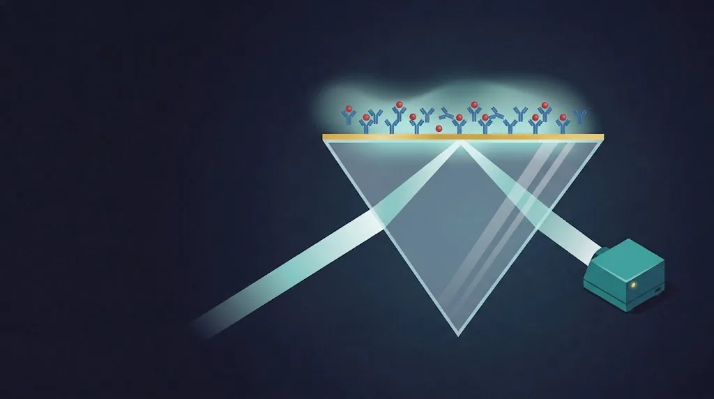
Light is shone through a glass prism onto a gold film about 50 nm thick. At one specific wavelength (or angle), the light couples into surface plasmons — charge oscillations at the metal surface — and the reflected light dips. When molecules bind on the gold, the local refractive index changes and that resonance shifts. The instrument tracks the shift in real time.
The Kretschmann configuration. Binding on the gold film changes the refractive index inside the evanescent field and shifts the resonance dip (solid → dashed).
Because the light never passes through the sample, SPR also works in complex matrices such as serum and plasma. For how this planar gold-film approach compares with nanoparticle-based localized SPR (LSPR), see LSPR vs SPR: pros and cons.
SPR measures a change in refractive index within roughly 200–300 nm of the sensor surface. In practice, that change tracks how much material is bound to the surface at each moment. Instruments report it as a shift in resonance wavelength (Δλ) or angle, often converted to response units (RU), and plot it against time.
SPR does not see individual molecules, and it does not need them to carry a label. It sees material arriving at and leaving the surface. More bound analyte gives a bigger signal, which is why the response grows with analyte concentration until the surface approaches saturation.
The flip side: anything that changes the refractive index of the solution itself also moves the signal. A mismatch between sample buffer and running buffer produces a "bulk" jump that is not binding. That is why SPR experiments use a reference channel — a surface without the specific ligand — and subtract it, leaving only the specific interaction.
A sensorgram is the plot of SPR response versus time, and it is the primary output of every SPR experiment. It shows whether an analyte binds the immobilized ligand and whether the binding is specific, and it contains the kinetic (kon, koff), affinity (KD) and concentration information you fit to extract numbers.
A typical kinetic sensorgram has five phases:
A phase-by-phase walkthrough, with what each shape means, is in SPR sensorgram explained. The technical version, including quality criteria for fitting, is TN-03: The SPR sensorgram explained.
SPR answers four questions about an interaction: does it happen and is it specific (specificity), how tightly do the partners bind (affinity, KD), how fast do they bind and release (kinetics, kon and koff), and how much analyte is in a sample (concentration). Which of these you get depends on how the experiment is set up.
For a worked example of setting up an experiment and extracting KD, see SPR for protein–protein interactions.
A typical SPR experiment takes one to three hours from bare sensor to result. Immobilizing the ligand takes about 30 minutes, the baseline then needs several minutes to settle, and a concentration series for one interaction takes roughly 30–60 minutes in static mode. Kinetic runs take longer, because each concentration adds a dissociation phase and usually a regeneration step.
Some reference points from our own protocols and application notes:
For a new interaction, most of the time goes into preparation rather than measurement: choosing the immobilization chemistry, scouting regeneration conditions and finding the right concentration range.
Besides the instrument, you need four things: a ligand (the molecule you immobilize), an analyte (its binding partner in solution), a sensor chip whose surface chemistry suits your ligand, and buffers — a running buffer, coupling and blocking solutions, and often a regeneration solution that resets the surface between cycles.
Choosing between covalent coupling and capture, and setting ligand density, is covered in detail in SPR surface chemistry: amine coupling vs. capture.
An SPR experiment follows the same basic steps on any instrument: prepare the sensor surface and immobilize the ligand, stabilize the baseline in running buffer, inject the analyte at increasing concentrations, regenerate the surface if needed, then subtract the reference channel and fit the responses to a binding model to get KD and, with flow, kon and koff.
A complete, instrument-level example — sensor, buffers, method and analysis — is the Starter Kit protocol.
In static SPR, the sample is injected by syringe into the flow cell and reaches the surface by diffusion; you read affinity (KD) from the steady-state plateau at each concentration. In flow (kinetic) SPR, a pump moves buffer continuously, so association and dissociation are both recorded, giving kon, koff, KD and Rmax.
Static SPR suits screening, specificity checks, quantification and affinity. The workflow is simpler and faster, and several samples can be compared side by side. The P4SPR 2.0 works this way: static SPR only, with four channels and no pump or fluidics, so there is nothing to clog.
Flow (kinetic) SPR adds the full kinetic profile, which matters when you need to understand binding mechanism or compare how long complexes stay bound. The P4PRO with the AffiPump runs both static and kinetic experiments on one instrument.
The two are complementary: static screening narrows candidates quickly, and kinetic analysis characterizes the most promising interactions in detail. The data behind this comparison are in Static vs. kinetic SPR: P4SPR 2.0 and P4PRO compared, with a one-page summary in the static vs. kinetic cheat sheet.
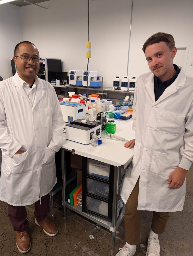
We've traveled to labs on four continents, and the most common thing we hear from our clients is: "I'm not sure my data is good enough." You're not alone — and you don't have to figure it out by yourself.
"We traveled to labs on four continents — and the most common thing we hear is: I'm not sure my data is good enough."
The top 3 issues we see in the field:
Why does the curve do that? What's with the sharp incline? Why doesn't the model fit? — these are the questions we live with. We wrote the cheat sheet so you don't have to guess.
"SPR would be the most appropriate — but we don't have in-house access."
We built the P4PRO to fit in a carry-on. We built our service model to fit your schedule. Whether you need full A-to-Z support or just a hand getting started — we know this instrument like the back of our hand, and we'll share everything we know.
Whether you're already part of the Affinité family or just starting to explore SPR — we'd love to hear from you.