Where the precision comes from

Overview

An SPR instrument never measures “binding” directly. It records light, finds the resonance in it, and follows where the resonance moves over time.

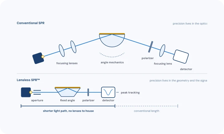
With no lenses (TN-03: Lensless optics and wavelength readout), much of the precision comes from how that data is processed, rather than from extra optics. This note explains how raw spectra become a sensorgram, where the precision comes from, and what really limits the smallest change you can see.

1 · WHAT THE DETECTOR RECORDS

Three ways to read a resonance

What arrives at the detector depends on the readout (TN-03: Lensless optics and wavelength readout). Wavelength readout fixes the angle and records a reflection spectrum, so the resonance is a dip at one wavelength. Angle readout fixes the wavelength and records reflected intensity across a range of angles, so the resonance is a dip at one angle.

Intensity readout fixes both and watches the brightness at a single working point on the side of the dip: the resonance shows up as a change in brightness, not a position. Our instruments use wavelength readout, and each channel delivers a full spectrum every second (up to five per second when a single channel is measured).

2 · FINDING THE RESONANCE

From a whole curve to one position

The resonance is a broad, smooth dip spread over many detector pixels. Its position can be found far more precisely than the pixel spacing, because the whole shape carries information, not just the darkest point. We call this step fit 1: it turns each spectrum into one precise position. How sharp the dip is, and so how precisely it can be found, starts at the chip (TN-05: The chip).

Common approaches: take the minimum of the raw curve (simple, but limited by pixel spacing and noisy); compute the centroid of the part of the dip below a threshold (robust and fast); or fit a function to the dip and read the position from the fit (precise when the model matches the shape). Each turns a whole curve into one number, the resonance position. Angle readout works the same way on a reflectivity-versus-angle curve.

Intensity readout skips the position. It is simple and fast, which suits imaging many spots at once, but it only works while the dip stays near the working point, and any change in light-source brightness reads as signal. In Affilabs.core, each channel’s full spectrum is tracked with methods tuned for the lensless signal, and the reference channel is subtracted in real time (TN-09: Getting a clean signal).

3 · FROM POSITION TO SENSORGRAM

Plotting the position over time

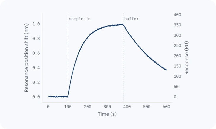
Plot the resonance position against time and you have the sensorgram: baseline, association, dissociation and regeneration (TN-10: From sensorgram to answer). Shifts are usually expressed in response units (RU), a scale proportional to the resonance shift; on our instruments, about 355 RU per nanometre. Fitting that curve for affinity and kinetics is the second fit (fit 2, TN-10: From sensorgram to answer).

For protein layers, the shift scales with the mass bound per area, which is what lets a sensorgram be read as “how much bound”.

4 · SENSITIVITY IS NOT RESOLUTION

Sensitivity, resolution and detection limit

Sensitivity is how far the resonance moves for a given refractive-index change. It is mostly set by physics: a gold film gives about 1800 nm/RIU near water. It is not constant: the resonance shifts more per refractive-index unit at longer wavelengths, so over bulk changes of about 0.01 RIU or more the response is no longer linear.

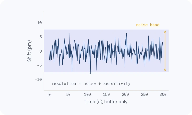
Resolution is the smallest change you can tell apart from noise: the noise divided by the sensitivity. The detection limit is the lowest analyte concentration that gives a resolvable shift. It depends on resolution and also on the assay: surface, analyte size and format (TN-06: The binding surface, TN-07: Designing a binding experiment).

Noise comes from the light source, the detector and temperature. Averaging more spectra lowers noise but blurs fast events: a 10-second average is quieter than a 1-second one, and it can miss a fast association. That is why the precision of an SPR instrument lives as much in its tracking as in its optics.