
IN SHORT
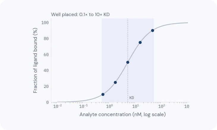
- Fit for affinity: plot the plateau height against concentration (TN-07: Designing a binding experiment); the concentration that gives half the maximum is the KD.
- Fit for kinetics: under flow (TN-08: Delivering the sample), the rise and fall of each curve show how fast it binds (kon) and lets go (koff); their ratio is KD.
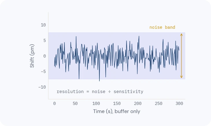
- Check the residuals: what is left after the fit should look like plain noise (TN-04: Where the precision comes from); a pattern means the model is wrong.
Overview
A sensorgram holds more than one answer: whether something binds, how strongly, how fast, and how much active material you have.
This note shows how to read the curve first, then fit it (fit 2; fit 1, in TN-04: Where the precision comes from, made each point), then check that the numbers can be trusted.
1 · READ THE CURVE
Read the curve before you fit it
A typical cycle has five phases.
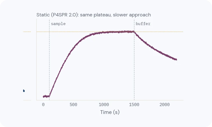
Baseline: running buffer over the surface, flat and stable; drift or spikes here mean the system isn’t ready (TN-09: Getting a clean signal). Association: the analyte is injected and the response rises as it binds. For a simple one-to-one interaction it curves smoothly towards a plateau; a nearly straight rise suggests mass transport (TN-08: Delivering the sample). Steady state: binding and release balance. This is an equilibrium, not necessarily a full surface.
Dissociation: buffer replaces the analyte and the response falls as complexes come apart. Regeneration: a short pulse, often low-pH glycine, removes what’s left and returns the baseline (TN-06: The binding surface).
Look for steps at the start and end of the injection (a bulk effect, removed by referencing), a baseline that doesn’t return, and a response that keeps rising with no plateau (non-specific binding). Fix those before fitting.

2 · AFFINITY FROM EQUILIBRIUM
Affinity from equilibrium
At each concentration, take the response at steady state, plot it against concentration, and fit a binding isotherm. KD is the concentration giving half the maximum response.
This works in static mode, because it needs equilibrium, not rates (TN-08: Delivering the sample). It is reliable when the series spans roughly 0.1–10× KD and each injection is close to equilibrium (TN-07: Designing a binding experiment).

3 · KINETICS
Kinetics from curve shapes
With controlled flow, the association and dissociation shapes give the rate constants: kon, how fast it binds, and koff, how fast it lets go (also written ka and kd), with KD = koff / kon. A one-to-one model is fitted to the whole concentration series at once.
Always look at the residuals, the difference between data and fit: they should look like plain noise (TN-04: Where the precision comes from). Systematic patterns, rather than noise, mean the model is wrong for this data: a heterogeneous surface or mixed analyte (two populations binding differently), avidity (a two-armed analyte holding on to two ligands, TN-07: Designing a binding experiment), or mass transport (TN-08: Delivering the sample).
A different model is only justified when it is physically plausible and the experiment supports it, not simply because it fits better.

4 · ACTIVE CONCENTRATION
Active concentration
Not every molecule in a protein prep binds: some are misfolded, aggregated or damaged. SPR can measure the active concentration, the amount that actually binds a given partner, which can differ from the total protein measured by absorbance.
It is a quality-control number, and it comes from the same curves: two lots with the same total protein can differ in activity.
5 · PLAUSIBILITY
Is the answer plausible?
A fit always returns numbers, even when the model is wrong or the data cannot support them. Before you report a KD or rate constants, check that they make sense.
Rmax. Compare the fitted maximum response with what the immobilized amount allows: Rmax ≈ (analyte molecular weight ÷ ligand molecular weight) × immobilized ligand response (RU) × binding sites per ligand. A fitted Rmax far above that points to non-specific binding or aggregation; far below points to an inactive, poorly oriented or crowded ligand.
Residuals. They should look like plain noise, with √χ² close to the noise floor (TN-04: Where the precision comes from). A pattern means the model is wrong for this data (section 3).
What the data can support. koff can only be measured if the signal visibly drops during dissociation; for very slow off-rates, make the dissociation phase longer. A KD needs concentrations spread around it, from a tenth to ten times, not all on the plateau (TN-07: Designing a binding experiment).
Self-consistency. The KD from the plateaus (section 2) should be close to koff/kon from the kinetic fit (section 3).
Replicates. The error a fit reports describes how well one curve was fitted, not how reproducible the result is. Report the spread across replicates, and say whether they are repeat injections or independent surfaces (TN-07: Designing a binding experiment).
Cross-check. Where possible, compare with an orthogonal method. Antibody levels measured on a P4SPR, for example, were cross-validated against ELISA.
The same ground in plainer words: SPR sensorgram explained walks through a curve phase by phase, and the sensorgram cheat sheet matches odd curve shapes to their fixes.
Related
TECH NOTE · TN-07
Designing a binding experiment
Ligand or analyte, the concentration series, controls and replicates.
TECH NOTE · TN-08
Delivering the sample: static and flow
Diffusion, flow and mass transport, and when static is enough.
TECH NOTE · TN-09
Getting a clean signal
Referencing, buffer matching, drift and complex samples: how to keep only the binding.